Display Imhist In App Designer Matlab

Image histograms with Matlab

Reading an image and getting information

To read images into the MATLAB environment you use the function imread, whose basic syntax is: imread('filename').

Other informative functions are: numel(f), to calculate the total number of pixels in the image; size(f), which gives the row and column dimensions of an image, in our example 576px X 809px; whos(f), function which displays additional information about an array. In our example, uint8 is one of the image classes supported by Matlab, indicating that unsigned 8-bit integers in the range [0,255] (1 byte per element) are used to represent pixel values.

Finally we display our test image with: imshow(f) .

Image histograms

The histogram of a digital image with the possible levels of intensity in the range [0, G] is defined as a discrete function:

h(rk)=nk

Where rk is the k-th intensity in the range [0, G] and nk is the number of pixels in the image where the intensity level is rk. The value of G is 255 for class uint8 (8 bits), and 65535 for images of class uint16 (16 bits). Note that G = L-1 for class uint8 and uint16.

Sometimes you need to work with normalized histograms, obtained simply by dividing all elements of h(rk) by the total number of pixels in the image, which we denote with n:

where k = 0, 1, 2, …, L-1. From probability theory, we recognize p(rk) is an estimate of the probability of occurrence of rk level intensity.

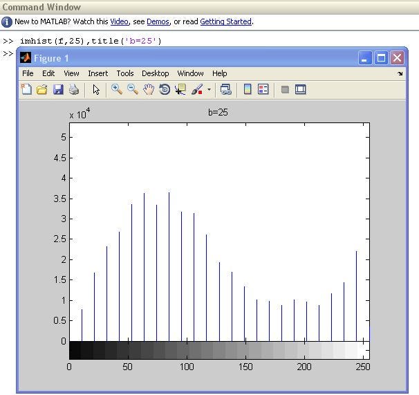
The main function of the toolbox to treat image histograms is imhist with the basic syntax:

h = imhist(f, b)

where f is the input image, h is its histogram, and b is the number of clusters used in forming the histogram (if b is not included, b = 256 is used by default. A cluster (bin) is simply a subdivision of the intensity scale. For example, if we are working with images uint8 and b=2, then the intensity scale is divided into two ranges: from 0 to 127 and from 128 to 255. The resulting histogram will have two values: h(1), equal to the number of pixels in the image with values in the range [0, 127] and h(2), equal to the number of pixels with values in the range [128, 255].

We get the normalized histogram using the espression:

p = imhist(f, b)/numel(f)

the numel(f) function gives the number of elements in the array f (i.e. the number of pixels in the image).

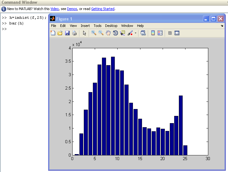
Bar histograms

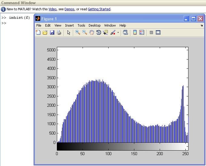
The easiest way to plot your histogram on the screen is to use imhist with no specified parameters: imhist(f). This is the histogram display default in the toolbox. However, there are many other ways to plot a histogram. Histograms can also be plotted using bar charts. To do this we can use the function:

bar(horz,z,w)

where z is a row vector containing the points for plotting, horz is a vector the same size of z that contains horizontal scale increases, and width is a number between 0 and 1. In other words, the values of horz give the horizontal increases and the values of z are the corresponding vertical values. If horz is omitted, the horizontal axis is divided in units from 0 to length(z). When width is 1, the bars touch each other; when is 0, the bars are just vertical lines. The default is 0.8.

When you print a bar graph, it is customary to reduce the resolution of the horizontal axis into bands. The following commands produce a bar chart with the horizontal axis divided into groups of about 10 levels:

» h=imhist(f, 25);

» horz=linspace( 0, 255, 25);

» bar(horz, h)

» axis([0 255 0 40000])

The fourth statement in the preceding code was used to expand the lower range of the vertical axis and to set the horizontal axis. One of the axis function syntax forms is:

axis([horzmin horzmax vertmin vertmax])

which sets the minimum and maximum values in the horizontal and vertical axes.

You can add a title to the chart using the function title, whose basic syntax is title('titlestring') where titlestring is a string of characters that will appear on the title, centered above the graph.

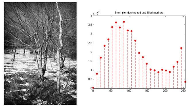
Stem plots

Another type of chart is stem, which is similar to a bar chart. The syntax is:

stem(horz,z,'LineSpec','fill')

where z is the row vector that contains plotting points and horz is the same as the function bar. If omitted, the horizontal axis is divided into units from 0 to length (z), as above. The third parameter LineSpec is a triplet of values that respectively indicate the color, the type of line drawn and the marker type that will be used.

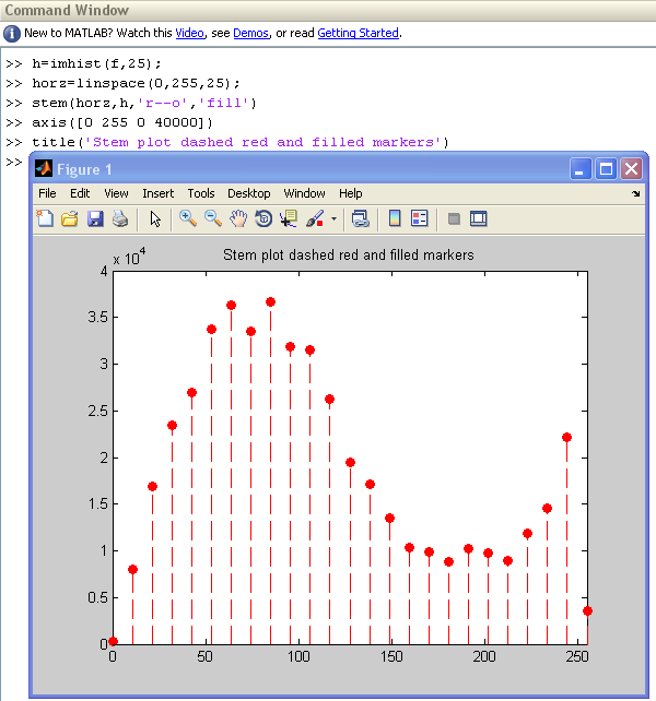
For example, stem(horz, h, r — o) produces a chart where lines and markers are red, lines are dashed and markers are little circles. If fill is used, the marker is filled with the color specified in the first element of the triplet.

In a next article, we will talk about histogram equalization, a simple way to increase the dynamic range of an image.